Troubleshooting transmission lines and passive RF parts

I have made some test measurements with a network analyzer, I would like to share my results and experiences in time dimensions measurements.

Instead of making measurements in frequency domain sometimes it’s worth switching into time domain. Newer network analyzers usually support this function, it’s called DTF (distance-to-fault). As its name suggests this type of measurement is capable of detecting the location of the failures in the transmission line system (e.g. damages, loose/soaked connectors). Sometimes regular measurement in frequency domain (e.g. Return Loss or VSWR) won’t show the real failure or they may suggest that everything is fine with the system. For instance if the attenuation of the cable is really high it can have a significant effect on the RL of the cable and antenna system – it may show that the RL is fine even if you place a short at the far end of the cable.

I’m going to describe which parameters should be set, and how to perform DTF and 1-port transmission measurements, it’s more or less the same with all VNAs. First the frequency range (start/stop frequency): it should be the same as the antenna’s bandwidth. Setting the frequency range correctly is crucial because it’ll define the fault resolution and the maximum distance. If the antenna’s bandwidth is narrow, sometimes it’s worth placing a 50 ohm load to the far end of the cable. The stop distance should be a bit higher than the cable’s length. Cable loss: it should be given in dB/m, it’s also important to give the accurate value. The cable loss will define the accuracy of the RL or VSWR values. Propagation velocity: a number between 0 and 1. It defines the speed of the EM signal within the transmission line in the unit of speed of light (that’s why it should be less than 1). The propagation velocity defines the accuracy of the fault location. These are the two parameters you should definitely look up in the cable’s data sheet.

After everything had been adjusted on the network analyzer, I assembled my test measurement setup: two 1.5 m coaxial transmission lines connected together ended with an 50 ohm load. So the setup is really simple but it shows how loose connectors or an unmatched load can influence the Return Loss. First I tightened the connectors properly and placed a load to the end, let’s see the results:

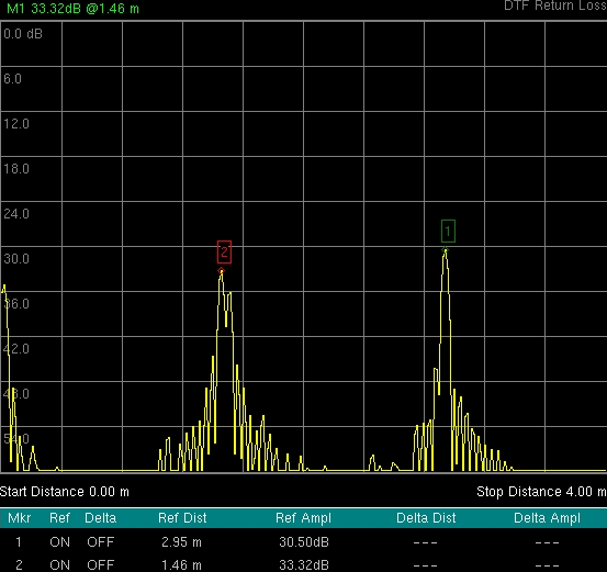
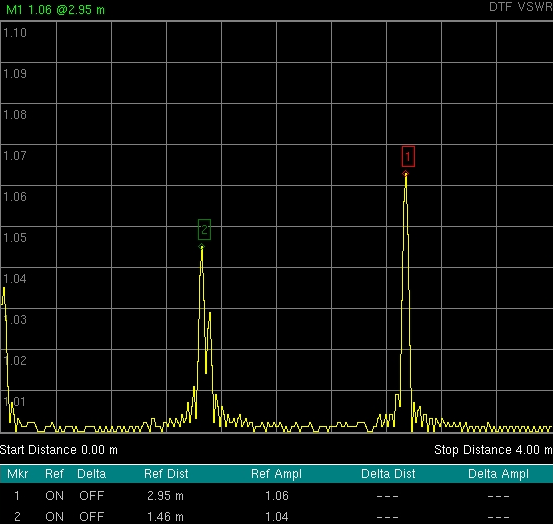
In the first picture the RL, in the second picture the VSWR can be seen as a function of distance. If everything was assembled appropriately I could measure around -30 dB RL (and the corresponding VSWR), which is excellent. Next I loosened the connectors between the two cables and at the load, you can probably guess which scenario belongs to which picture.

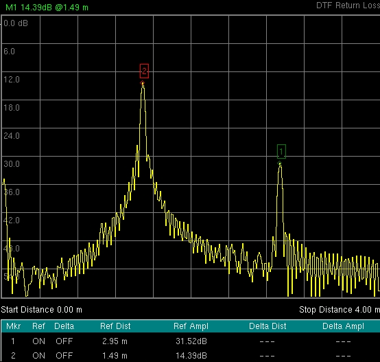
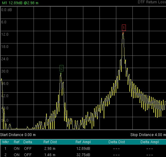
A -12 dB RL is still considered a good value, but you can see how a bad connector can affect the measured values.

Next I measured the cable’s attenuation using 1-port attenuation measurement. Instead of using both ends of the cable – like the traditional 2-port transmission measurement – which is sometimes unfeasible, the cable’s attenuation can be measured with the help of one port. It can be achieved by placing a short (or an open, but I prefer short) to the far end of the cable causing total reflection.

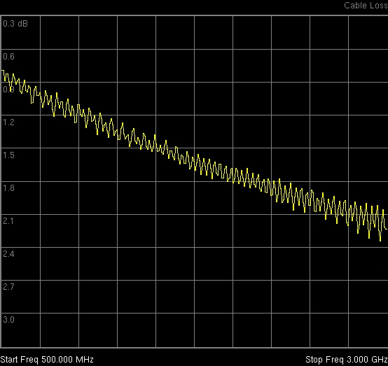
Maybe I should’ve applied a bit more smoothing, but it’s linear function: as frequency increases so does the attenuation. To make sure the measurement is accurate (but this result seems correct to me) I inserted an attenuator of 10 dB: I expect the signal above to drop by 10 dB.

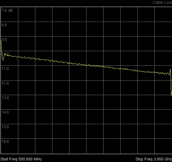
So the 1-port cable loss measurement works appropriately, we don’t need to connect the far end of the cable to the network analyzer.